In my previous review series, I wrote a brief review of set theory. This time around we’ll take a look at the binary tree data structure. The tree structure is very common, incredibly useful data structure in the field of computer science and it’s essential that any engineer understand how they work.
The Tree Data Structure
A tree, unlike some other data structures, such as an array, linked list, stack, or queue, is a hierarchical data structure. Each entry in the tree is called a node and the topmost node in the tree is called the root of the tree (or the root node). The elements that are directly under a node are referred to as child nodes and the node that the children fall under is called a parent node.
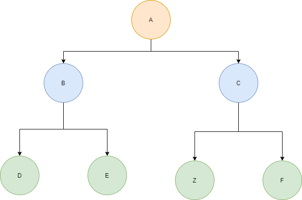
Let’s look at an example of what a tree might look like:
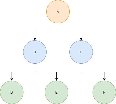
In this example, A is the root of the tree. The nodes B and C are children of A and A is the parent of B and C. Similarly, D and E are children of B and F is a child of C.
Nodes that do not have any children are called leaves in the tree. In this example, D, E, and F are leaves.
The height of a tree is defined as the longest path from the root node to any leaf node in the tree. The height of our example tree is 2.
The tree above is an example of a specific type of tree, known as a binary tree. A binary tree is a tree structure whose elements have at most two children. Since each element in a binary tree can only have at most two children, we often just refer to them as the left child and the right child.
The rest of this review will focus primarily on binary trees due to their usefulness throughout computer science.
Representing a Tree
Trees are extremely easy data structures to implement in a programming language. When you break it down, a tree is just composed of a collection of nodes. Each node contains the following attributes:
- A data value
- A pointer to the left child
- A pointer to the right child
That’s it! So, it should hopefully become pretty clear that we could implement a tree node in C as follows:
1struct Node {
2    int data;
3    struct Node* left;
4    struct Node* right;
5};
So, let’s create our example tree from the previous section in C:
 1#include <stdlib.h>
 2// Represents a node in a tree
 3typedef struct Node {
 4    char data;
 5    struct Node* left;
 6    struct Node* right;
 7} Node;
 8int main(int argc, char* argv[])
 9{
10    // Build the root node on the heap
11    Node* root = malloc(sizeof(Node));
12    root->data = 'A';
13    root->left = malloc(sizeof(Node));
14    root->right = malloc(sizeof(Node));
15    // Build the rest of the tree
16    root->left->data = 'B';
17    root->right->data = 'C';
18    root->left->left = malloc(sizeof(Node));
19    root->left->left->data = 'D';
20    root->left->right = malloc(sizeof(Node));
21    root->left->right->data = 'E';
22    root->right->right = malloc(sizeof(Node));
23    root->right->right->data = 'F';
24    return 0;
25}
While this may not be the most elegant code every, it’s simply to illustrate how the tree structure works.
Properties of Binary Trees
There are a few important properties of binary trees that are worth knowing. I won’t be going into proofs of any of these properties. We’ll leave that as an exercise for the reader.
The Maximum Number of Nodes at any Given Level
How would one go about computing the maximum number of nodes at any given level, l, in a binary tree? Well, it’s simply:
$$2^l$$
So, for the root node (level 0), the max number of nodes is 20 = 1, which should make perfect sense, and the max number for level 1 would be 21 = 2.
The Maximum Number of Nodes for a Tree of a Given Height
Let’s say that you had a tree of some height, h. You could determine the maximum number of nodes that would fit in this binary tree with the following:
$$2^h - 1$$
So, if I had a tree with a height of 4, the maximum number of nodes in that tree would be:
$$2^4 - 1 = 15$$
The Minimum Height of a Tree with n Nodes
Say that I know that I have a tree with some number of nodes, n. I can compute the minimum height of that tree with:
$$\mid \, \log_{2}(n+1) \mid \, - 1$$
Types of Binary Trees
We’ve already discussed that binary trees are a specific kind of tree, but it turns out there are a few different forms of binary trees. Let’s take a look at some of these forms:
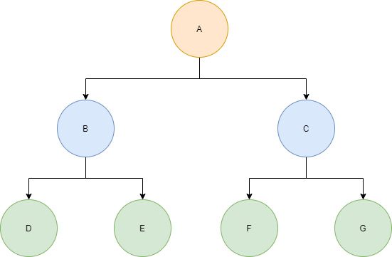
Full Binary Tree
A binary tree is considered to be a full binary tree simply if every node in the tree has 0 or 2 children. Here’s an example:
Complete Binary Tree
A binary tree is said to be a complete binary tree if all the levels, except potentially the last level, are completely filled and all the nodes are as far left as possible. Here’s an example:
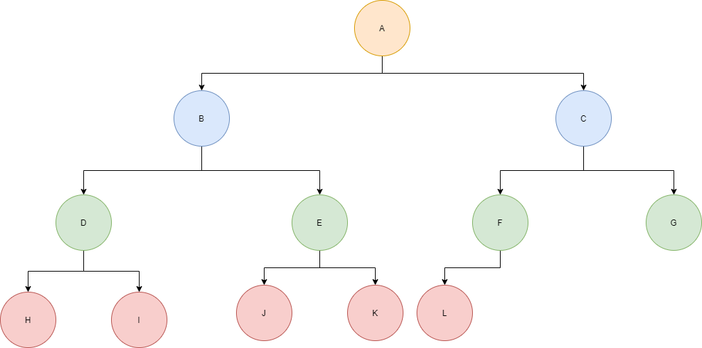
A great practical example of a complete binary tree structure would be a binary heap.
Perfect Binary Tree
A binary tree is a perfect binary tree if all of the internal nodes in the tree have two children and all of the leaf nodes are on the same level. Here’s an example:
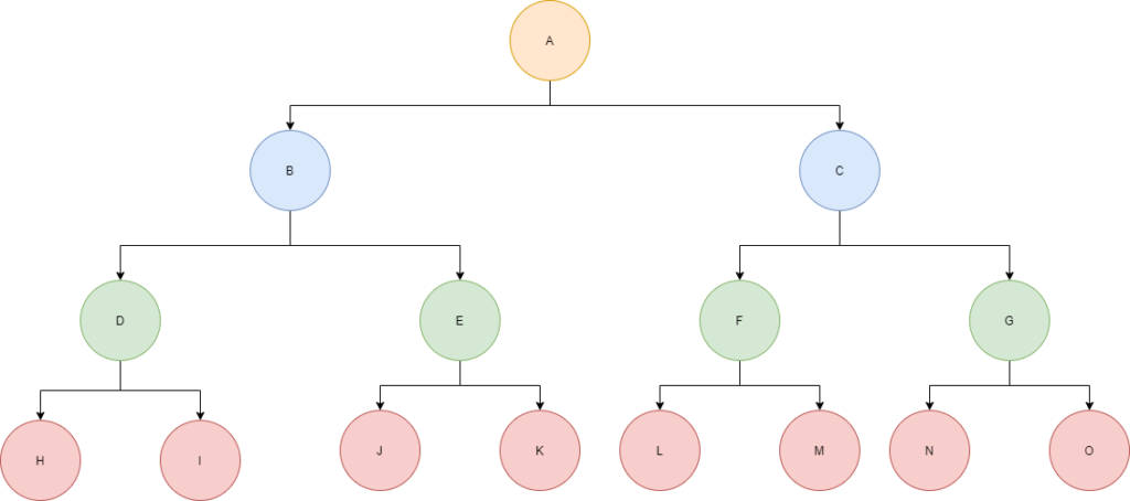
It’s worth noting a couple of interesting properties of a perfect binary tree. First, if L is the number of leaf nodes in the tree and I is the number of internal nodes, then
$$L = I + 1$$
Also, the number of nodes for a perfect binary tree of height h is:
$$n = 2^{h+1} - 1$$
Balanced Binary Tree
A balanced binary tree is a binary tree who’s height is
$$O(\log_{2}n)$$
where n is the number of nodes in the tree. A simplified version of this definition is that a balanced binary tree is a binary tree in which the depth of the two sub-trees for every node never differ by more than 1.
So, a simple example of a balanced binary tree would be:

There are a number of specific tree implementations that result in a balanced binary tree. For example, red-black trees are self-balancing binary trees that maintain their O(log n) height by ensuring that the number of black nodes on each root to leaf path is equal and that there are no adjacent red nodes. AVL trees maintain the O(log n) height constraint by ensuring that the difference between heights of the left and right sub-trees is at most 1 (like in our simplified definition above).
The reason one might want to concern themselves with maintaining a balanced binary tree is because they provide O(log n) time for search, insert, and delete operations.
Pathological Trees
A pathological tree (also known as a degenerate tree) is a tree in which every internal node only has one child. Here’s a simple example:
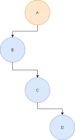
It’s also worth noting that, in terms of performance, this is identical to a linked list, which should make sense if you think about it.
Tree Traversal
An important topic when discussing trees is how to go about traversing them. Unlike a linear data structure, such as an array, there are a number of logical approaches. We will look at the most common of these here.
Consider the following tree:
There are two primary ways to traverse a tree: depth-first and breadth-first. The depth-first method is further divided into 3 (primary) methods for traversing the tree:
- Inorder Traversal (Left sub-tree, root, right-subtree): D B E A C F
- Preorder Traversal (Root, left sub-tree, right sub-tree): A B D E C F
- Postorder Traversal (Left sub-tree, right-subtree, root): D E B F C A
The breadth-first approach, also known as the level-order traversal, would result in the following: A B C D E F.
Let’s look at an example of how we can do these various traversals in code. For fun, I’ll do this example in Java:
 1package com.hackeradam.traversal;
 2import java.util.Queue;
 3import java.util.LinkedList;
 4// Represents a node in a binary tree
 5class Node
 6{
 7    // The data stored in this node
 8    public char data;
 9    // References to the left and right node, respectively
10    public Node left;
11    public Node right;
12    public Node(char data) {
13        this.data = data;
14        left = right = null;
15    }
16}
17// Represents a binary tree data structure
18class BinaryTree
19{
20    // The root node in the tree
21    Node root;
22    public BinaryTree() {
23        root = null;
24    }
25    // Prints the tree using postorder traversal
26    public void printPostorder(Node node) {
27        if (node == null) // base case
28            return;
29        // Start with the left sub-tree
30        printPostorder(node.left);
31        // Then do the right sub-tree
32        printPostorder(node.right);
33        // Then print the node
34        System.out.print(node.data + " ");
35    }
36    // Prints the tree using inorder traversal
37    public void printInorder(Node node) {
38        if (node == null) // base case
39            return;
40        // Start with the left sub-tree
41        printInorder(node.left);
42        // Then handle the node
43        System.out.print(node.data + " ");
44        // Finally handle the right sub-tree
45        printInorder(node.right);
46    }
47    // Prints the tree using preorder traversal
48    public void printPreorder(Node node) {
49        if (node == null) // base case
50            return;
51        // Start with this node
52        System.out.print(node.data + " ");
53        // Then do the left sub-tree
54        printPreorder(node.left);
55        // Then the right sub-tree
56        printPreorder(node.right);
57    }
58    // Prints the level order traversal
59    public void printLevelOrder() {
60        Queue<Node> q = new LinkedList<Node>();
61        q.add(root);
62        while (!q.isEmpty()) {
63            // Remove the head of the queue and print it
64            Node tmp = q.poll();
65            System.out.print(tmp.data + " ");
66            // Enqueue the left sub-tree
67            if (tmp.left != null)
68                q.add(tmp.left);
69            // Then the right sub-tree
70            if (tmp.right != null)
71                q.add(tmp.right);
72        }
73    }
74}
75public class Main {
76    public static void main(String... args) {
77        // Build the binary tree from the example
78        BinaryTree tree = new BinaryTree();
79        tree.root = new Node('A');
80        tree.root.left = new Node('B');
81        tree.root.left.left = new Node('D');
82        tree.root.left.right = new Node('E');
83        tree.root.right = new Node('C');
84        tree.root.right.right = new Node('F');
85        System.out.print("Inorder Traversal: ");
86        tree.printInorder(tree.root);
87        System.out.println();
88        System.out.print("Preorder Traversal: ");
89        tree.printPreorder(tree.root);
90        System.out.println();
91        System.out.print("Postorder Traversal: ");
92        tree.printPostorder(tree.root);
93        System.out.println();
94        System.out.print("Level Order Traversal: ");
95        tree.printLevelOrder();
96        System.out.println();
97    }
98}
Again, this isn’t necessarily the most elegant code. It’s just here to illustrate a point.
You’ll notice that the level order traversal is a bit more complicated and uses a queue data structure. You can also achieve the same result by printing each level of the tree, but I find the queue approach to be more elegant.
Anyway, the general algorithm is as follows:
- Create a new empty queue
- enqueue the root node
- Loop while tmp != null
- Remove a node from the queue and store in tmp
- print tmp->data
- enqueue the left-child of tmp
- enqueue the right-child of tmp
This is, in my opinion, an easy and more elegant solution than the alternative of iterating over each level of the tree and printing it.
Insertion with Level Order Traversal
Let’s say that I had a binary tree and I wanted to insert a node into the first available position in level order. I could do this by performing a level order traversal of the tree. If we come across a node who has no left-child, we insert the new node there, otherwise we insert it at the first node that has no right child.
So, let’s again consider this example tree:
If I were to insert a node, say ‘Z’, into this tree, it would become the following:
Now that we understand the principle, let’s see how we could add a level order insertion method to the example code from above:
 1// Inserts an item into the tree using level order traversal
 2    public void insert(Node item) {
 3        if (root == null) {
 4            root = item;
 5            return;
 6        }
 7        // Do the level order traversal
 8        Queue<Node> q = new LinkedList<Node>();
 9        q.add(root);
10        while (!q.isEmpty()) {
11            Node tmp = q.poll();
12            if (tmp.left == null) {
13                // Insert the node here
14                tmp.left = item;
15                break;
16            } else {
17                // else, enqueue the left node
18                q.add(tmp.left);
19            }
20            if (tmp.right == null) {
21                // insert the node here
22                tmp.right = item;
23                break;
24            } else {
25                // else, enqueue the right node
26                q.add(tmp.right);
27            }
28        }
29    }
Deletion from a Binary Tree
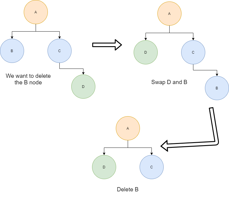
Let’s say that you have a binary tree in which you want to delete a node in such a way that the tree shrinks from the bottom up (note that this is not the same as deletion in a binary search tree!). In other words, the deleted node will be replaced by the bottom-most and right-most node.
Consider this example tree:

If we were to delete the ‘B’ node using this method, we would get the following result:

The algorithm for this works as follows:
- Start at the root node and find the deepest, right-most node in the binary tree and the node that we want to delete
- Replace the deepest, right-most node with the node to be deleted
- Delete the deepest, right-most node
So, for our above example, The process looks something like this:
Now that we understand the mechanics of this deletion method, let’s take a look at how we could add it to our Java example code:
 1// Deletes the deepest node in the tree
 2    void deleteDeepestNode(Node target) {
 3        Queue<Node> q = new LinkedList<Node>();
 4        q.add(root);
 5        // Find the deepest node and delete it
 6        Node tmp = null;
 7        while (!q.isEmpty()) {
 8            tmp = q.poll();
 9            if (tmp == target) {
10                tmp = null;
11                return;
12            }
13            if (tmp.right != null) {
14                if (tmp.right == target) {
15                    tmp.right = null;
16                    return;
17                } else {
18                    q.add(tmp.right);
19                }
20            }
21            if (tmp.left != null) {
22                if (tmp.left == target) {
23                    tmp.left = null;
24                    return;
25                } else {
26                    q.add(tmp.left);
27                }
28            }
29        }
30    }
31    // Deletes the given item in the binary tree as outlined above
32    void delete(char item) {
33        if (root == null)
34            return; // Nothing to do
35        if (root.left == null && root.right == null) {
36            if (root.data == item)
37                root = null; // Delete the root node
38            return;
39        }
40        // Find the target node and the last node
41        Queue<Node> q = new LinkedList<Node>();
42        q.add(root);
43        Node target = null;
44        Node tmp = null;
45        while (!q.isEmpty()) {
46            tmp = q.poll();
47            if (tmp.data == item) // We found the target node, store it
48                target = tmp;
49            if (tmp.left != null)
50                q.add(tmp.left);
51            if (tmp.right != null)
52                q.add(tmp.right);
53        }
54        if (target != null) {
55            target.data = tmp.data;
56            deleteDeepestNode(tmp);
57        }
58    }
That’s All… For Now
That’s all I have to say about trees in this post. Stay tuned for future posts where we will explore Binary Search Trees, AVL Trees, and Red Black Trees!